Coursera 강의 “Machine Learning with TensorFlow on Google Cloud Platform” 중 다섯 번째 코스인 Art and Science of Machine Learning의 강의노트입니다.
Regularization
-
The
simplerthe better -
Factor in model complexity when calculating error
- Minimize: loss(Data|Model) + complexity(Model)
- loss is aimed for low training error
- but balance against complexity
-
Optimal model complexity is data-dependent, so requires hyperparameter tuning
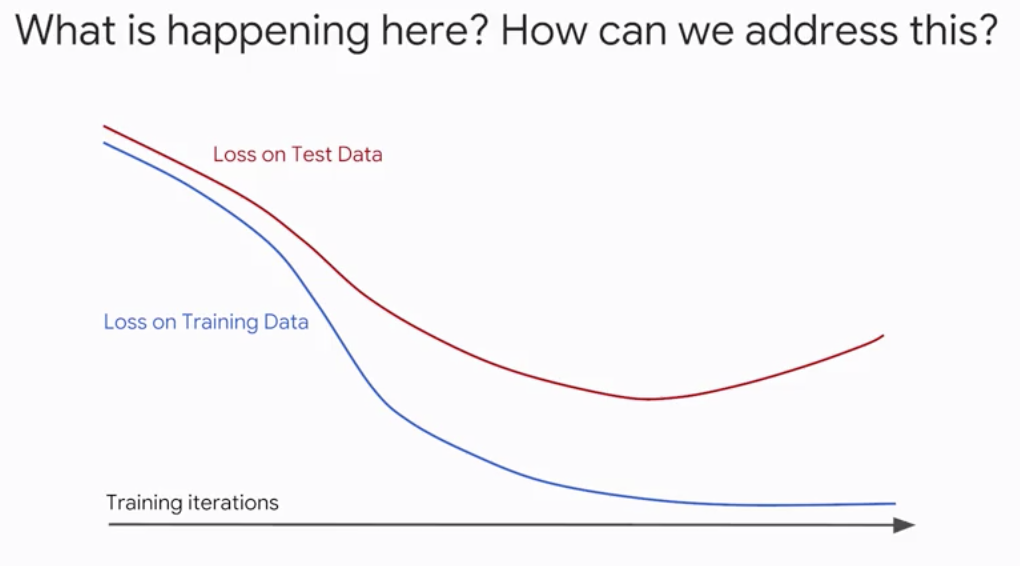
Regularizationis a major field of ML research - Early Stopping
- Parameter Norm Penalties
L1 / L2 regularization- Max-norm regularization
- Dataset Augmentation
- Noise Robustness
- Sparse Representations
- …
L1 & L2 Regularizations
- How can we measure model complexity?
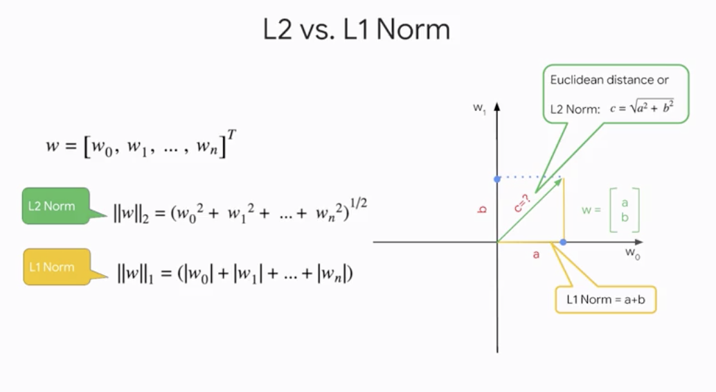
L2 vs. L1 Norm
-
In
\[L(w,D)+\lambda||w||_{\color{Red}2}\]L2regularization,complexityof model is defined by the L2 norm of the weight vectorlambdacontrols how these are balanced
-
In
\[L(w,D)+\lambda||w||_{\color{Red}1}\]L1regularization,complexityof model is defined by the L1 norm of the weight vector- L1 regularization can be used as a
feature selectionmechanism
- L1 regularization can be used as a
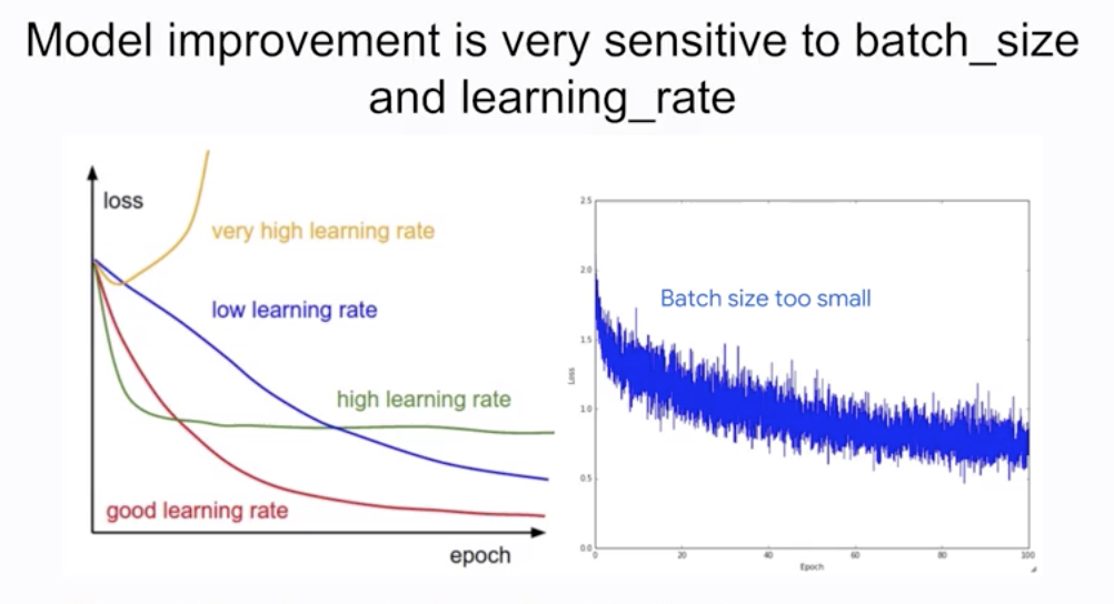
Learning rate and batch size
- We have several knobs that are
dataset-dependent Learning ratecontrols the size of the step in weight space- If too
small, training will take alongtime - If too
large, training willbouncearound - Default learning rate in Estimator’s LinearRegressor is smaller of 0.2 or
1/sqrt(num_features)→ this assume that your feature and label values are small numbers
- If too
- The
batch sizecontrols the number of samples that gradient is calculated on- If too
small, training willbouncearound - If too
large, training will take a verylongtime 40 - 100tends to be a good range for batch size Can go up to as high as 500
- If too
- Regularization provides a way to define model complexity based on the values of the weights
Optimization
Optimizationis a major field of ML researchGradientDescent— The traditional approach, typically implemented stochastically i.e. with batchesMomentum— Reduces learning rate when gradient values are smallAdaGrad— Give frequently occurring features low learning ratesAdaDelta— Improves AdaGrad by avoiding reducing LR to zeroAdam— AdaGrad with a bunch of fixesTtrl— “Follow the regularized leader”, works well on wide models- …
- Last two things are good defaults for
DNN and Linearmodels
Practicing with TensorFlow code
- How to change optimizer, learning rate, batch size
train_fn = tf.estimator.inputs.pandas_input_fn(..., batch_size=10)
myopt = train.FtrlOptimizer(learning_rate=0.01,
l2_regularization_strength=0.1)
model = tf.estimator.LinearRegressor(..., optimizer=myopt)
model.train(input_fn=train_fn, steps=10000)- Control
batch sizevia the input function - Control
learning ratevia the optimizer passed into model - Set up
regularizationin the optimizer - Adjust number of steps based on batch_size, learning_rate
- Set number of steps. not number of epochs because distributed training doesn’t play nicely with epochs.
Hyperparameter Tuning
- ML models are mathematical functions with parameters and hyper-parameters
Parameterschanged during model trainingHyper-parametersset before training
- Model improvement is very sensitive to batch_size and learning_rate
- There are a variety of model parameters too
- Size of model
- Number of hash buckets
- Embedding size
- Etc.
- Wouldn’t it be nice to have the NN training loop do meta-training across all these parameters?
- How to use
Cloud ML Enginefor hyperparameter tuning- Make the parameter a command-line argument
- Make sure outputs don’t clobber each other
- Supply hyperparameters to training job
Regularization for sparsity
-
Zeroing outcoefficients can help with performance, especially with large models and sparse inputs- Fewer coefficients to store / load → Reduce memory, model size
- Fewer multiplications needed → Increase prediction speed
- L2 regularization only makes weights small, not zero
-
Feature crosseslead to lots of input nodes, so having zero weights is especially important -
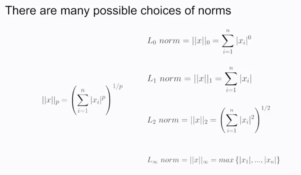
L0-norm(the count of non-zero weights) is an NP-hard, non-convex optimization problem -
L1 norm(sum of absolute values of the weights) is convex and efficient; it tends to encourage sparsity in the model -
There are many possible choices of norms
-
\[L(w,D)+\lambda_1\sum^n|w|+\lambda_2\sum^nw^2\]Elastic netscombine the feature selection of L1 regularization with the generalizability of L2 regularization
Logistic Regression
- Transform linear regression by a sigmoid activation function
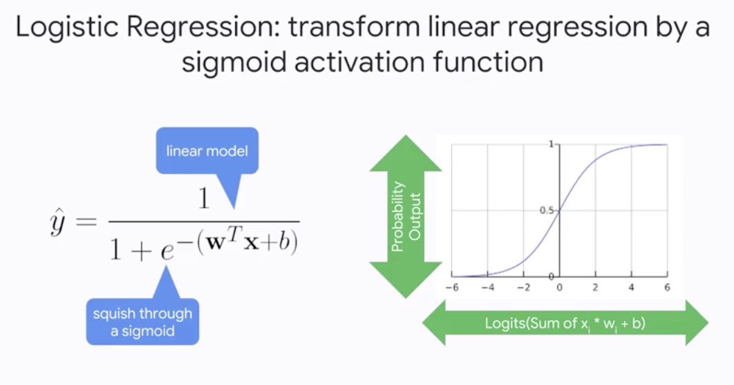
Logistic Regression
-
The output of Logistic Regression is a calibrated probability estimate
- Useful because we can cast
binary classificationproblems intoprobabilisticproblems: Will customer buy item? becomes Predict the probability that customer buys item
- Useful because we can cast
-
Typically, use
cross-entropy(related to Shannon’n information theory) as the error metric- Less emphasis on errors where the output is relatively close to the label.
-
Regularizationis important in logistic regression because driving the loss to zero is difficult and dangerous- Weights will be driven to -inf and +inf the longer we train
- Near the asymptotes, gradient is really small
-
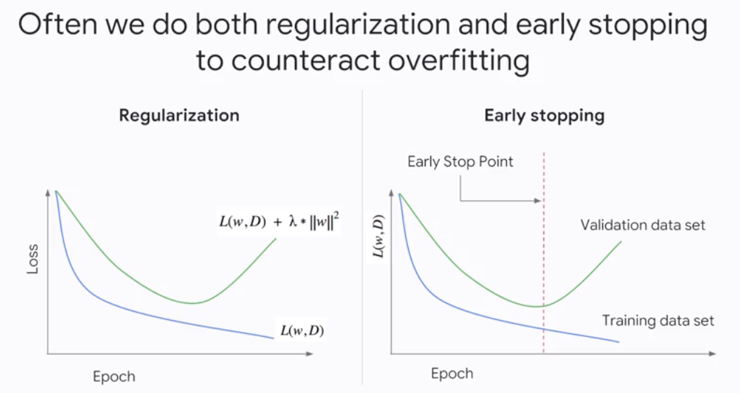
Often we do both
regularizationandearly stoppingto counteract overfitting
- In many real-world problems, the probability is not enough; we need to make a
binary decision- Choice of
thresholdis important and can be tuned
- Choice of
- Use the
ROC curveto choose the decision threshold based on decision criteria
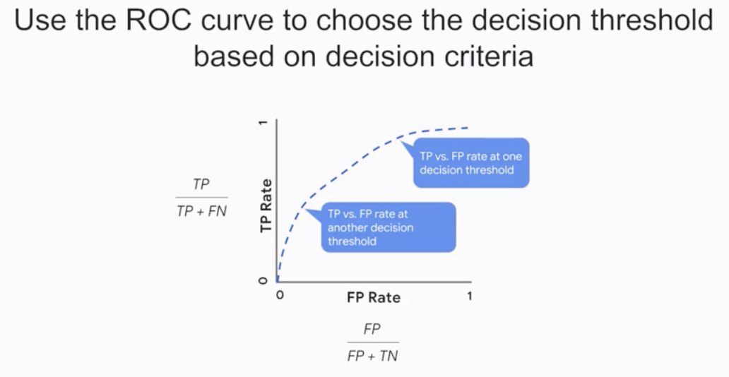
- The
Area-Under-Curve(AUC)provides an aggregate measure of performance across all possible classification thresholds- AUC helps you choose between models when you don’t know what decision threshold is going to be ultimately used.
- “If we pick a random positive and a random negative, what’s the probability my model scores them in the correct relative order?”
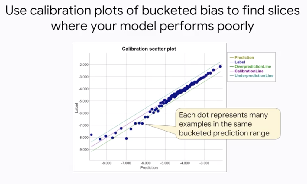
- Logistic Regression predictions should be
unbiased- average of predictions == average of observations
- Look for bias in slices of data. this can guide improvements
- Use calibration plots of bucketed bias to find slices where your model performs poorly
Neural Networks
- Feature crosses help linear models work in nonlinear problems
- But there tends to be a limit…
Combine featuresas an alternative to feature crossing- Structure the model so that features are combined Then the combinations may be combined
- How to choose the combinations? Get the model to learn them
- A Linear Model can be represented as nodes and edges
- Adding a Non-Linearity
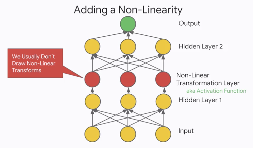
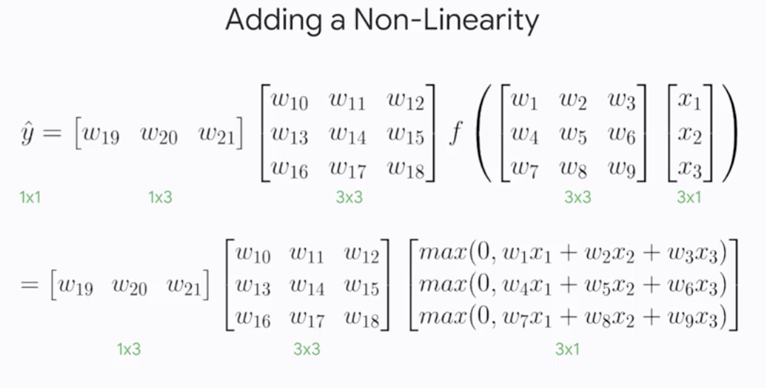
- Our favorite non-linearity is the
Rectified Linear Unit(ReLU)
-
There are many different ReLU variants
\[Softplus = ln(1+e^x)\] \[Leaky ReLU=f(x)=\begin{cases}0.01x&for&x>0\\x&for&x\le0\end{cases}\] \[PReLU=f(x)=\begin{cases}\alpha x&for&x>0\\x&for&x\le0\end{cases}\] \[ReLU6=min(max(0,x),6)\] \[ELU=f(x)=\begin{cases}\alpha (e^x-1)&for&x>0\\x&for&x\le0\end{cases}\] -
Neural Nets can be
arbitrarily complex- Hidden layer - Training done via BackProp algorithm: gradient descent in very non-convex space
- To increase
hidden dimension, I can addneurons - To increase
function composition, I can addlayers - To increase
multiple labels per example, I can addoutputs
Training Neural Networks
- DNNRegressor usage is similar to LinearRegressor
myopt = tf.train.AdamOptimizer(learning_rate=0.01)
model = tf.estimator.DNNRegressor(model_dir=outdir,
hidden_units=[100, 50, 20],
feature_colimns=INPUT_COLS,
optimizer=myopt,
dropout=0.1)
NSTEPS = (100 * len(traindf)) / BATCH_SIZE
model.train(input_fn=train_input_fn, steps=NSTEPS)- Use
momentum-basedoptimizers e.g. Adagrad(the default) or Adam. Specify numberof hidden nodes.- Optionally, can also regularize using
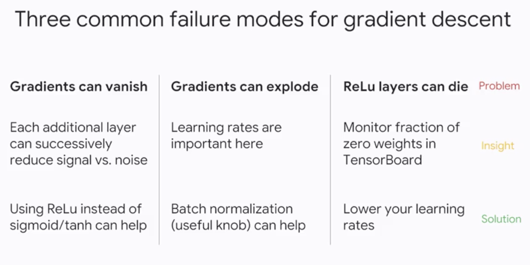
dropout - Three common failure modes for gradient descent
- There are benefits if feature values are
smallnumbers- Roughly zero-centered, [-1, 1] range often works well
- Small magnitudes help gradient descent
convergeand avoid NaN trop Avoiding outliervalues helps with generalization
- We can use standard methods to make feature values
scale to small numbers- Linear scaling
- Hard cap (clipping) to max, min
- Log scaling
Dropoutlayers are a form of regularization
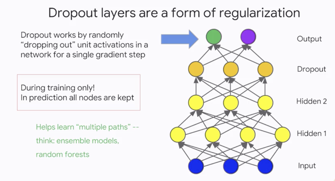
- Dropout simulates
ensemblelearning - Typical values for dropout are between
20 to 50percent - The
moredrop out, thestrongerthe regularization- 0.0 = no dropout regularization
- Intermediate values more useful, a value of dropout=0.2 is typical
- 1.0 = drop everything out! learns nothing
- Dropout acts as another form of
Regularization. It forces data to flow downmultiplepaths so that there is a more even spread. It also simulatesensemblelearning. Don’t forget to scale the dropout activations by the inverse of thekeep probability. We remove dropout duringinference.
Multi-class Neural Networks
- Logistic regression provides useful probabilities for
binary-classproblems - There are lots of
multi-classproblems- How do we extend the logits idea to multi-class classifiers?
- Idea: Use separate output nodes for each possible class
- Add additional constraint, that total outputs = 1.0
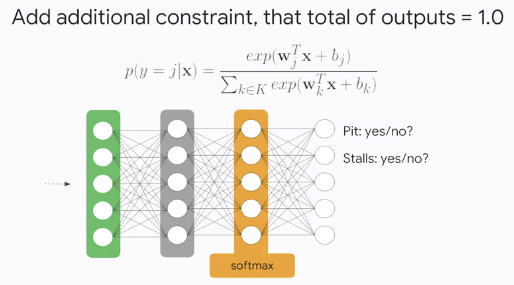
- Use one
softmaxloss for all possible classes
logits = tf.matmul(...) # logits for each output node -> shape=[batch_size, num_classes]
labels = # one-hot encoding in [0, num_class] -> shape=[batch_size, num_classes]
loss = tf.reduce_mean(
tf.nn.softmax_cross_entropy_with_logits_v2(
logits, labels) # shape=[batch_size]
}- Use sotfmax only when classes are
mutually exclusive- “Multi-Class, Single_label Classification”
- An example may be a member of only one class.
- Are there multi-class setting where examples may belong to more than one class?
tf.nn.sigmoid_cross_entropy_with_logits(logits, labels) # shape=[batch_size, num_classes]- If you have hundreds or thousands of classes, loss computation can become a significant
bottleneck- Need to evaluate every output node for every example
- Approximate versions of softmax exist
- Candidate Sampling calculates for all the positive labels, but only for a random sample of negatives:
tf.nn.sampled_softmax_loss - Noise-contrastive approximates the denominator of softmax by modeling the distribution of outputs:
tf.nn.nce_loss
- Candidate Sampling calculates for all the positive labels, but only for a random sample of negatives:
- For our classification output, if we have both mutually exclusive labels and probabilities, we should use
tf.nn.softmax_cross_entropy_with_logits_v2. - If the labels are mutually exclusive, but the probabilities aren’t, we should use
tf.nn.sparse_softmax_cross_entropy_with_logits. - If our labels aren’t mutually exclusive, we should use
tf.nn.sigmoid_cross_entropy_with_logits.